
Transient detection#
Why transient detection?#
The indicator brightness rises and falls with whichever underlying biological signal the indicator is engineered to report (intracellular calcium for GCaMP, extracellular dopamine for sensors like dLight, and so on for serotonin, acetylcholine, voltage, and the rest of the indicator catalog). A brief, large upward deflection in the trace therefore corresponds to a brief, large excursion in that local signal: a bout of population activity, a transmitter release event, or a shift in release-uptake balance, depending on which indicator is in use.
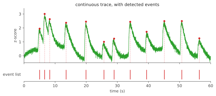
Transient detection (also called peak detection) is the analysis that extracts the times of those deflections. The resulting event list is useful for relating activity to other observables (behavioral timestamps, drug administration, sensory stimuli, signals recorded simultaneously from other regions), for aggregating into a session-level event rate or mean amplitude that compares across conditions, and for cross-correlating event streams between regions to extract timing relationships independent of slow shared drift.
Detecting transients#
The basic detector is conceptually simple. To flag samples that are anomalous relative to the rest of the trace, we characterize that trace by two summary numbers: a typical level and a noise scale (how far a typical sample sits from the typical level). Each peak more than K noise scales above the typical level is counted as a transient, where K is a sensitivity multiplier the user chooses (larger K means fewer detections of any kind, real or noise; values around 3 are typical in photometry). The output is a discrete list of (time, amplitude) events extracted from a continuous recording.
Importantly, the detector runs on the preprocessed fluorescence trace, not on the raw recording. Two upstream cleanup steps are typically applied first: an isosbestic correction that removes optical artifacts shared between the indicator-sensitive and isosbestic channels, and z-score normalization that puts the trace on a noise-relative scale where detection thresholds are interpretable across recordings. What survives is, in principle, a trace whose deflections are predominantly indicator-driven; the detector takes that on faith and operates on whatever comes out of preprocessing.
The following sections cover how to improve this basic approach to deal with complications that arise out of the characteristics of the signal.
Addressing drift#
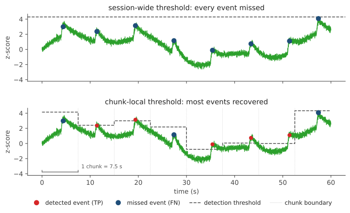
The mean of the signal is non-stationary across the session. Slow processes that survive preprocessing (residual photobleaching, slow patchcord motion, hemodynamic effects, and genuine biological state changes) create a long-term drift that breaks any single threshold applied across the session. A naive fixed threshold therefore catches events on stretches where the baseline is high and misses events on low-baseline stretches, simply because the threshold doesn’t move with the drift.
One way of addressing the session drift is to split the signal into contiguous chunks of fixed duration and recompute the typical level and noise scale from the samples inside each chunk. The detection threshold within a chunk is then tailored to that chunk’s local conditions. The robust pair to use here is the median for the typical level and MAD (the median absolute deviation) for the noise scale, the same pair introduced in the z-score explainer.
Addressing outlier-induced bias#
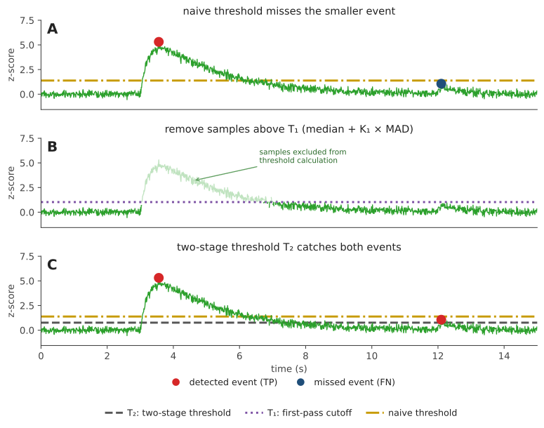
Even with a reasonable window, the chunk’s typical level and noise scale are still sensitive to what samples happen to land in it. A chunk that catches a large event plus its slow decay tail, or two events arriving close together, sees those high-amplitude samples shift the typical level slightly upward and inflate the noise scale substantially (their distance from the typical level is large, so they enter the spread tally at full distance). Both shifts push the detection threshold upward, and smaller real events in the same chunk fall below it.
A one-sided trim of the per-chunk samples addresses this. Before computing the noise reference for a chunk, blank the upward outliers, presumed to be event-driven rather than noise-driven, and recompute the noise reference on what remains. The trimmed samples still participate in detection (they are not removed from the chunk, only from the noise reference). The remaining samples produce a cleaner estimate of the underlying noise scale, and the threshold set against that estimate catches smaller events that the contaminated single-pass version would miss.
In compact form the procedure is:
Compute the median and MAD of the raw chunk. Form the first-pass cutoff T₁ = median + K₁ × MAD.
Set aside samples above T₁. These are presumed extreme upward outliers. The filter is one-sided: downward excursions (e.g. a brief loss of coupling) are not removed.
Recompute the median and MAD on the remaining samples. Form the detection threshold T₂ = median′ + K₂ × MAD′.
In the original chunk (including the samples trimmed for the noise estimate), mark every sample exceeding T₂. These are the detected transients.
K₁, K₂ are the multipliers: how many noise scales above the median each threshold sits.
T₁ = median + K₁ × MAD is the first-pass cutoff; raw-chunk samples above it are excluded from the noise reference.
T₂ = median′ + K₂ × MAD′ is the detection threshold, applied against the cleaned median and MAD.
Conceptually, K₁ (e.g. 2) places the cutoff T₁ a couple of noise-scales above the median: high enough to clear the noise, low enough that real events fall above it and get trimmed. K₂ (e.g. 3) then sets the detection threshold T₂ on the cleaned estimate. A higher K₂ is a stricter “what counts as a real event” criterion (fewer detections, real or noise), a lower one more permissive.
Reading the output#
The detector returns a per-event list of (time, amplitude) pairs plus two per-recording summary scalars:
Event rate (events per minute): how often the detector flags a transient. An approximation of the underlying biological event rate, dependent on the noise floor (which sets where the threshold lands) and contaminated by some non-zero rate of noise crossings.
Mean amplitude (in noise-relative units, i.e. multiples of the chunk’s noise scale): the average above-threshold excursion among detected events. An approximation of the average biological event size, expressed in units that are local to the recording’s noise floor.
Rate is the headline statistic in most photometry papers that quantify transients: it is the single number that gets compared across conditions (control versus drug, baseline versus learning, etc.). The two dependencies above (noise floor across recordings; noise-crossing contribution within a recording) are unpacked next.
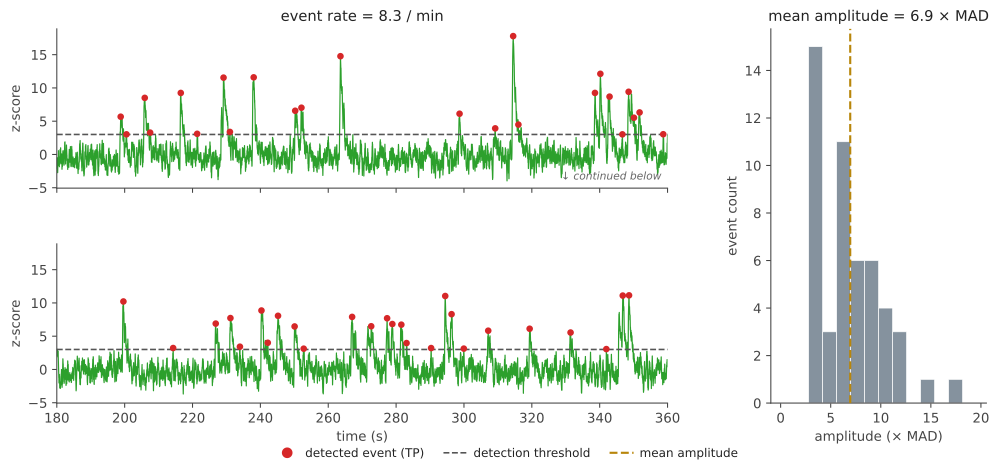
Mean amplitude is reported in noise-relative units, so cross-recording comparisons silently assume that the recordings have matched noise floors: the same physical event reads as a smaller noise-scale multiple when the noise floor is higher. The z-score explainer covers this fragility at session scale; the same logic applies here at chunk scale, and the same workarounds apply (re-express amplitudes in dF/F, or argue that SNR is matched).
Within a single recording, some fraction of the detected rate is noise rather than biology. Any finite threshold is crossed by chance, so even a recording with no biological transients sits at a non-zero noise floor of detections, and a low rate should be read against that floor rather than as biology.